Coastal Erosion
A number of complex, dynamic models are available for examining processes related to sediment transport, wave energy effects, beach profile changes, and so on. While the rigour of such models is clearly an advantage for predicting physical changes and examining coastal processes, their application is severely limited for assessments in many countries, for two reasons. First, such models often demand good quality, high resolution data for a range of variables and model parameters. Good quality data is often very limited and therefore the range of methods for assessing the impacts of climate and sea-level changes is also restricted. Second, the more complex coastal models are not well suited to addressing the issues of sea-level rise because very different time and space scales are involved. In such circumstances, the detailed processes and predictive accuracy of the model may be less important than the capability to conduct simulations for the purpose of examining model sensitivities and uncertainties under sets of “what if” scenarios on coarse temporal and spatial scales.
Consequently, following the guidance given in the USCSP Handbook (Benioff et al., 1996, Chapter 5.5) and the UNEP Handbook (Feenstra et al., 1998), a variant of the ‘Bruun Rule’ (Bruun, 1962) was developed at the International Global Change Institute (IGCI) at the University of Waikato, New Zealand. This method appears suitable for simulating shoreline changes on beach and dune systems.
The basic Bruun Rule
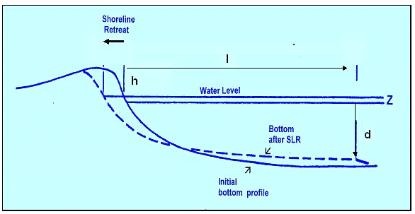
The concept behind the 2-dimensional “Bruun Rule” model is explained in the USCSP Handbook (Benioff et al., 1996). In effect, in the Bruun Rule the equilibrium profile of a beach-and-dune system is re-adjusted for a change in sea level (see Figure 1). A rise in sea level will cause erosion and re-establishment of the equilibrium position of the shoreline further inland, as follows:
Ceq = z l / (h + d) where:
Ceq is the equilibrium change in shoreline position (in metres)
z is the rise in sea level (in metres)
l is the closure distance (the distance offshore to which materials are transported and “lost”, in metres)
h is the height in metres of the dune at the site
d is the water depth in metres at closure distance ( l/(d+h) thus gives slope)
Principles of the Bruun Rule as the basis for the coastal impact model
There are two important drawbacks to using this simple model to examine shoreline change under a trend of rising sea level. First, it gives only the “equilibrium” (or steady-state) change. In reality, coastal systems do not adjust instantaneously; rather, there is apt to be some time lag in the response. Second, in reality shoreline retreat, as evidenced by historical data on beach profiles, is apt to occur in “fits and starts” over time, not as a steady, year-by-year incremental change. This uneven response of the shoreline is partly a function of the chance occurrence of severe stormy seasons, which often cause erosion (in contrast, a season of very few, or mild, storms may allow the natural system to replenish the sediment supply and the shoreline to advance).
For these reasons, the Bruun Rule was modified slightly to add a response time and a stochastic “storminess” factor as follows:
dC/dt = (Ceq – C)/+ S where:
t is time (years)
C is the shoreline position (metres) relative to that of t=0
Ceq is the equilibrium value of C
is the shoreline response time (years)
S is a stochastically-generated storm erosion factor
In other words, the yearly change in shoreline is a function of the difference between where the shoreline should be (according to the Bruun Rule) in that year and where it actually is (as a consequence of what has occurred in previous years), as well as the effect of storms. The greater the difference, the greater the potential erosion in that year, subject to the rapidity at which the system can respond.
The concept was incorporated into a costal impact model. The model is forced by changes in sea level (projections selected by the user from library files) and by the randomly selected “stormy seasons”, as defined by the user. The model runs on yearly time-steps and the results are displayed graphically.